FORMULA TO REVERSE DIGITS IN A CELL

I explored a lot on internet for a customized formula which can reverse the digits in a cell and found many solutions using VBA user defined function or by installing add-in but couldn't find any help with excel formula. So here is the formula for it that I developed after 3 hours of struggle:)

=SUMPRODUCT(MID(A1,ROW(INDIRECT("1:"&LEN(A1))),1)*1,POWER(10,ROW(INDIRECT("1:"&LEN(A1)))-1)) 

Please post in comment section if you have some other short and simple way to do it.

Thanks!

MAKE NEXT CONTROL VISIBLE ONCE THE FOCUS LOSES FROM FIRST CONTROL (KEYDOWN EVENT)

Below is the code to make next textbox visible once you finish typing in first textbox and press enter key or tab.

Controls on my form:

4 labels:                     lblCode, lblName, lblDept and lblDesig

4 textboxes:               txtCode, txtName, txtDept and txtDesig

1 CommandButton:   cmdSubmit

First I have made all the controls invisible except first textbox and label (lblcode & txtcode in my case) while loading the userform.

Private Sub UserForm_Initialize()

Me.txtCode.SetFocus

Me.txtName.Visible = False

Me.txtDept.Visible = False

Me.txtDesig.Visible = False

Me.lblName.Visible = False

Me.lblDept.Visible = False

Me.lblDesig.Visible = False

Me.cmdSubmit.Visible = False

End Sub

Only the first textbox and label will be visible when userform loads.

Below code on KeyDown Event of txtCode will make next set of controls (lblName & txtName) visible when you press enter key or tab key after typing in first textbox (txtCode) and set the focus on txtName.

Private Sub txtCode_KeyDown(ByVal KeyCode As MSForms.ReturnInteger, ByVal Shift As Integer)

If KeyCode = vbKeyReturn Or KeyCode = vbKeyTab Then

        If txtCode.Text <> vbNullString Then

            txtName.Visible = True

            lblName.Visible = True

            txtName.SetFocus

        End If

End If

End Sub

Below code on KeyDown Event of txtName will make next set of controls (lblDept & txtDept) visible when you press enter key or tab key after typing in second textbox (txtName) and set the focus on txtDept.

Private Sub txtName_KeyDown(ByVal KeyCode As MSForms.ReturnInteger, ByVal Shift As Integer)
If KeyCode = vbKeyReturn Or KeyCode = vbKeyTab Then
    If txtName <> vbNullString Then
        txtDept.Visible = True
        lblDept.Visible = True
        txtDept.SetFocus
    End If
End If
End Sub

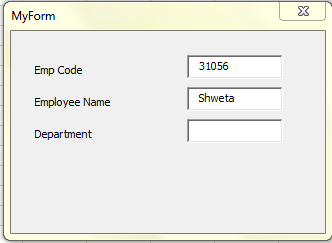
Below code on KeyDown Event of txtDept will make next set of controls (lblDesig & txtDesig) visible when you press enter key or tab key after typing in third textbox (txtDept) and set the focus on txtDesig.

Private Sub txtDept_KeyDown(ByVal KeyCode As MSForms.ReturnInteger, ByVal Shift As Integer)

If KeyCode = vbKeyReturn Or KeyCode = vbKeyTab Then

    If txtDept <> vbNullString Then

        txtDesig.Visible = True

        lblDesig.Visible = True

        txtDesig.SetFocus

    End If

End If

End Sub

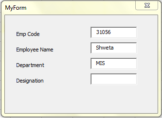
Below code on KeyDown Event of txtDesig will make next control (cmdSubmit) visible when you press enter key or tab key after typing in last textbox (txtDesig) and set the focus on cmdSubmit.

Private Sub txtDesig_KeyDown(ByVal KeyCode As MSForms.ReturnInteger, ByVal Shift As Integer)

If KeyCode = vbKeyReturn Or KeyCode = vbKeyTab Then

    If txtDesig <> vbNullString Then

        cmdSubmit.Visible = True

        cmdSubmit.SetFocus

    End If

End If

End Sub

vbKeyReturn - Enter key on your keyboard

vbKeyTab - Tab key on your keyboard

For more Key Code Constants you can refer to Microsoft site using this link.

Key Code Constants

Thanks.

CALCULATE TOTAL NUMBER OF A WEEKDAY IN A MONTH

Cell D2 : Data validation for Month Name
Cell E2: Data validation for Weekday Name

Formula in F2:
=SUMPRODUCT(--(WEEKDAY(ROW(INDIRECT(DATE(YEAR(D2),MONTH(D2),1)&":"&EOMONTH(D2,0))))=MATCH(E2,{"Sunday","Monday","Tuesday","Wednesday","Thursday","Friday","Saturday"},0)))

Note: Make sure the month name list (A2:A13 in my case) that you are using for data validation, is in date format, not in text format.

Is the post helpful?

Please post your valuable comment. Thanks!

CALCULATE SHIFT HOURS FROM SHIFT WINDOW (START TIME AND END TIME)

Say, you are given shift timings ( shift start time and shift end time) and you need to calculate shift hours from them. Below is the formula for that.

Formula in B2:
=MOD(RIGHT(A2,5)-LEFT(A2,5),1)*24 and drag it down.

RESTRICT USER TO MOVE YOUR USERFORM

Use below codes to restrict the users to move your userform.

1) Declare variables

Private m_sngAnchorLeft As Single
Private m_sngAnchorTop As Single
Private m_blnSetAnchor As Boolean


2) Paste the below code in the Activate event of the userform

Private Sub UserForm_Activate()
If Me.Visible Then
        If Not m_blnSetAnchor Then
            m_sngAnchorLeft = Me.Left
            m_sngAnchorTop = Me.Top
            m_blnSetAnchor = True
        End If
    End If
End Sub

3) Paste the below code in the Deactivate event of the userform

Private Sub UserForm_Deactivate()
m_blnSetAnchor = False
End Sub

4) Paste the below code in the Layout event of the userform

Private Sub UserForm_Layout()
If m_blnSetAnchor Then
        Me.Left = m_sngAnchorLeft
        Me.Top = m_sngAnchorTop
    End If
End Sub

Note: All the above codes should be used

DISABLE CLOSE("X") BUTTON OF USERFORM

To disable the close(X) button of userform paste the below code on the QueryClose event of your userform.


Private Sub UserForm_QueryClose(Cancel As Integer, CloseMode As Integer)
If CloseMode = 0 Then
Cancel = True
MsgBox "The X is disabled, please use a button on the form.", vbCritical
End If
End Sub

CREATE FUNNEL CHART USING FORMULA

Following are the Steps:

1. Sort your data in Descending Order
2. Enter formula in C2  =REPT("|",B2/50) and drag it down
3.Choose the color that you want.